#Introduction
A data structure is a logical construct used to organize and store data in a way that enables efficient processing. Understanding the available structures helps you choose the right one for a given problem. My goal is not to give an algorithms course, but to detail some of the implementations Microsoft chose when building the .NET Framework classes, so you can pick the one that best fits your needs. If you want to learn more about how a particular data structure works, search for its name online.
#The notations
To measure the efficiency of an algorithm, we measure the time it takes. This is done by counting instructions and weighting them by their cost. There are several types of operations:
- Arithmetic operations
- Read / assign variables
- Comparisons
- …
To express algorithmic complexity, we use Big O notation. O(n) represents the worst-case scenario. Here are some examples. Imagine we have a list containing 1 million elements. If an algorithm is
- O(1): Whatever the number of elements, the time is always identical.
- O(ln(n)): For our list, it means that ln(1000000)≈14 operations to realize the algorithm
In order of complexity (from the fastest to the slowest): 1, ln(n), n, n ln(n), n2, en
#LinkedList<T>
It is a doubly linked circular list. This allows head and tail insertions in O(1). To insert at the tail, you simply insert before the head element since the list is circular. Searching requires traversing the entire list item by item, which is not efficient.
#List<T>
This is a dynamically resizing array. The default initial capacity is 4. When you insert an element while the array is full, a new array twice the size is allocated. The existing items are copied to the new array, and the new item is added. To insert at a specific index, all subsequent elements must be shifted one position to make room. Removal shifts all subsequent items left. Searching requires iterating through the entire list item by item, which is not efficient.
#SortedList<TKey, TValue>
Its operations are identical to those of List. However, items are kept sorted in ascending order. When adding an item, a binary search (O(log(n))) is used to find its correct position. The remaining insertion and removal operations are identical to those of an unsorted list.
#HashSet<T>
HashSet is implemented as a hash table that resolves collisions using coalesced chaining. To insert an element, it first computes the hash value using the GetHashCode method, then derives the array index as the hash modulo the array size. If that position is already occupied (a collision), the chaining mechanism kicks in: an empty bucket is found from the end of the table and the element is placed there. The original position stores a link pointing to that bucket. To find an element, its hash is computed and the element at the corresponding index is retrieved. If it matches the target value, the search is done. Otherwise, if a collision link exists, it is followed. This continues until a match is found or there are no more links. A hash function is considered good if no more than 5 elements in the collection share the same hash value. On average, the search is O(1). However, if the hash function is poor and generates many collisions, the search can degrade to O(n).
#Dictionary<TKey, TValue>
The dictionary works like HashSet, except that the hash value is computed from the key (TKey) rather than the value (TValue).
#SortedSet<T>
The SortedSet is implemented with a Red-Black tree (or two-color tree). This is a balanced search binary tree. All operations are done in O(log(n)).
#SortedDictionary<TKey, TValue>
In short, it is a SortedSet<KeyValuePair<TKey, TValue>>, and therefore shares the same behavior as SortedSet.
#Summary
##Insert item
| General | Head | Tail |
|---|
| LinkedList | O(n) | O(1) | O(1) |
| List | O(n) | O(n) | O(1) |
| SortedDictionary | O(log(n)) | N/A | N/A |
| Dictionary | O(1) | N/A | N/A |
| HashSet | O(1) | N/A | N/A |
| SortedSet | O(log(n)) | N/A | N/A |
| SortedList | O(n) | N/A | N/A |
##Remove item
| General | Head | Tail |
|---|
| LinkedList | O(n) | O(1) | O(1) |
| List | O(n) | O(n) | O(1) |
| SortedDictionary | O(log(n)) | N/A | N/A |
| Dictionary | O(1) | N/A | N/A |
| HashSet | O(1) | N/A | N/A |
| SortedSet | O(log(n)) | N/A | N/A |
| SortedList | O(n) | N/A | N/A |
##Get by index
| General |
|---|
| LinkedList | O(n) |
| List | O(1) |
| SortedList | O(1) |
##Get by value
| General |
|---|
| LinkedList | O(n) |
| List | O(n) |
| SortedDictionary | O(log(n)) |
| Dictionary | O(1) |
| HashSet | O(1) |
| SortedSet | O(log(n)) |
| SortedList | O(log(n)) |
#Measures
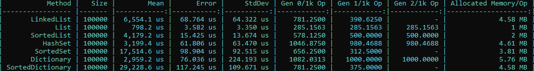
##Add First

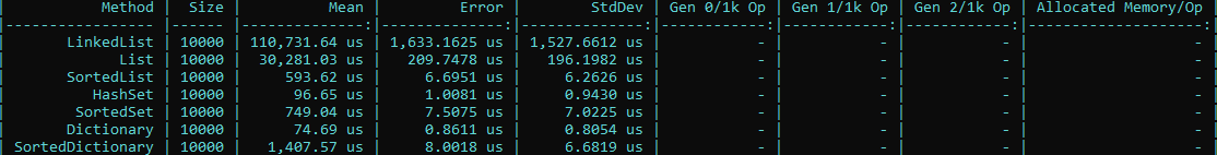
##Add Last
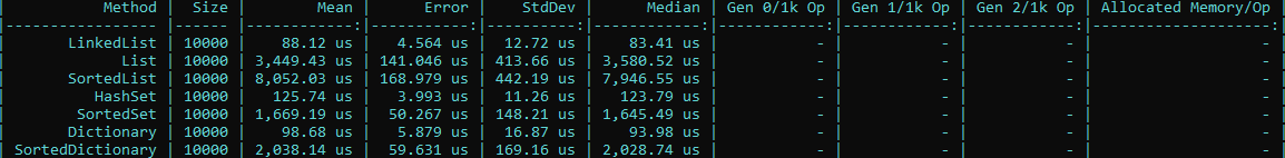
##Contains
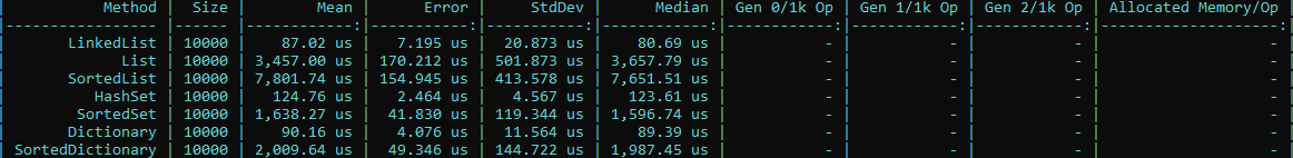
##Remove First
##Remove Last
#Conclusion
I hope this post has shown that each data structure serves a different purpose, with strong performance for certain operations and weaker performance for others. Choose the right one based on your specific needs.
Source code of the tests: Test Performance
Do you have a question or a suggestion about this post? Contact me!